Improving XVA Accuracy with Empirical Martingale Simulation

by Stefano Renzitti

Computing and risk managing XVAs for a bank's entire portfolio is a huge computational burden. Infrastructure constraints and calculation windows require banks to make tradeoffs between accuracy and calculation time, typically resulting in the use of significantly fewer Monte Carlo paths than would otherwise be used in a typical front office pricing application. This reality places more emphasis on the quality of the simulations being used to obtain the Monte Carlo estimates.

Over the years, many variance reduction techniques have been developed to help improve the Monte Carlo accuracy for a fixed number of simulation paths. In our previous paper [1], we demonstrated the use of one such technique where the pseudo random numbers were replaced with more carefully chosen quasi random numbers (Sobol' sequences from Broda's 65536 generator [2], randomized, and with a Brownian bridge path construction), resulting in significant error reductions at roughly the same computational cost.

In our latest paper [3], and with a similar objective, we explored another variance reduction technique called empirical martingale simulation (EMS) [4], where the underlying simulated risk factors' drifts are adjusted to ensure the linear instruments used to hedge the XVAs are reproduced exactly (martingales), no matter how many Monte Carlo paths are used. When these adjusted risk factors were used to compute the forward mark to markets of the portfolios, and ultimately the XVAs, we found that the Monte Carlo errors were on average reduced, in some cases, dramatically.

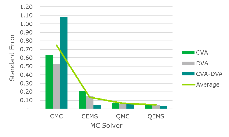
Figure 1 contains a summary of the CVA, DVA, and CVA-DVA Monte Carlo standard errors per $10,000 notional (results for FCA, FBA, and FCA-FBA were similar, respectively, so were omitted for brevity), for various portfolios of pay-fixed interest rate swaps (in, at, and out of the money; with sensitivities to 1, 6, and 11 currencies) computed using 1,024 paths (on the low end of what is typically used in practice), a local cross currency Hull White model for each counterparty (local in the sense that it only captures the risk factors underlying a particular netting set), and four Monte Carlo simulation techniques:

1. CMC: Classical Monte Carlo simulation with pseudo random numbers.

2. CEMS: CMC + EMS applied to the underlying simulated numeraire, exchange rates, and zero bonds.

3. QMC: Quasi Monte Carlo with the Brownian bridge path construction.

4. QEMS: QMC + EMS applied to the underlying simulated numeraire, exchange rates, and zero bonds.

Figure 1: CVA, DVA, CVA-DVA Monte Carlo standard errors per $10,000 USD notional, using 1,024 paths, by solver type, for various portfolios of interest rate swaps using local cross currency Hull White models.

The findings suggest that:

1. EMS provides a large error reduction (82% on average) when applied to risk factors generated with pseudo random numbers (compare CMC to CEMS on the Average series in Figure 1).

2. QMC provides a larger, less variable, error reduction (91% on average when compared to CMC) than CEMS, with the exception being for the CVA-DVA (and FCA-FBA) metrics, which were superb with both EMS based techniques.

3. EMS provides a more modest, but still impressive, error reduction (26% on average) when applied to risk factors generated with high quality quasi random numbers (compare QMC to QEMS). The combination produces the smallest overall errors, with an incredible 94% error reduction over CMC (on average).

Further inspection revealed that the benefits of applying EMS were concentrated in the more linear test cases, i.e.: DVA in out of the money portfolios, CVA in in the money portfolios, and CVA-DVA in all portfolios held against counterparties of similar credit quality as the bank. The utility gained from the approach therefore heavily depends on 1) the quality of the random numbers used to generate the risk factors, 2) the bank's portfolio composition, and 3) how much weight they place on the individual metrics (CVA, DVA) versus the netted metrics (CVA-DVA), where the latter netted metric may be more important to banks that report firm wide values, as defined in [5], and/or hedge the net non-credit market risk, for example.

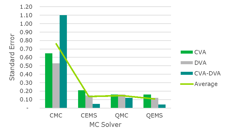
In our second set of tests, we switched from the low dimension local models (capturing 1, 6, and 11 currencies, respectively, using on average 11 factors per time step) to a high dimension global model (capturing 36 currencies with 71 factors per time step). Global models are typically used for cross-netting set consistency, operational simplicity, and/or entity-level calculations. In comparison to the local model QMC results, the global model QMC results deteriorated significantly (as expected due to higher dimensionality), while the CMC and CEMS results were unaffected, bringing the average QMC error in line with the average CEMS error (80% error reduction on average), see Figure 2. Fortunately, an application of EMS to the global model QMC risk factors provided an additional 27% error reduction on average, which is similar to the additional reduction obtained when applying EMS to the local model QMC risk factors (26% on average). QEMS therefore remains the best Monte Carlo solver tested. For the global model setting, the QEMS errors are tied with QMC errors and smaller than CEMS errors for CVA, smaller than both CEMS and QMC errors for DVA, and in line with CEMS errors and significantly smaller than QMC errors for CVA-DVA.

Figure 2: CVA, DVA, CVA-DVA Monte Carlo errors per $10,000 USD notional, using 1,024 paths, by solver type, for various portfolios of interest rate swaps using a global cross currency Hull White model set up to simulate 36 currencies.

In conclusion, dramatic error reductions over CMC can be obtained with either applying EMS, yielding approximately an 80% error reduction, or by switching to QMC, giving approximately a 90% error reduction for local models and an 80% error reduction for global models. An additional, more modest but still impressive, error reduction of approximately 25% (over QMC) emerges when combining QMC with EMS. Solving for the number of CMC paths that are needed to match CMC errors to the errors obtained with the other three Monte Carlo solvers (using 1024 paths), we get a clearer picture of just how impressive the efficiency gains are:

1. CEMS with 1,024 paths produces errors similar in size to CMC with 31k paths when using both local and global models.

2. QMC with 1,024 paths produces errors similar in size to CMC with 142k paths when using local models, and 27k paths when using the global model.

3. QEMS with 1,024 paths produces errors similar in size to CMC with 262k paths when using local models, and 51k paths when using the global model.

As we increased the number of paths from 1,024 to more commonly used values (2,048+), the efficiency gained from the two QMC based methods over the other two methods (CMC and CEMS) grew due to their enhanced order of convergence (0.70+ for local models, 0.60+ for global models, compared to 0.50 for CMC and CEMC). Generally, modeling the (mean squared) Monte Carlo error as a power law in the number of simulation paths, QMC tends to increase the order of convergence while EMS improves the rate of convergence. Using both ensures the results start in a good place and improve as quickly as possible with each additional simulation path used, helping to make more efficient use of a limited XVA computational budget.

For a more detailed description of the methodology, tests, convergence results for sensitivities, and the dependence of the results on portfolio characteristics, we refer the reader to the research paper [3]:

[1] Renzitti, S., Bastani, P., and Sivorot, S.. 2020. Accelerating CVA and CVA Sensitivities Using Quasi-Monte Carlo Methods. Wilmott Magazine 108, 78-93.
[2] http://www.broda.co.uk/
[3] Renzitti, S., Bastani, P., and Sivorot, S.. 2021. XVA Estimates with Empirical Martingale Simulation. Wilmott Magazine, Forthcoming. Preprint available at https://papers.ssrn.com/abstract=3948228
[4] Duan, J.C. and Simonatro, J.G.. 1998. Empirical martingale simulation for asset prices. Management Science, 44(9):1218-1233.
[5] Andersen, L., Duffie, D., and Song, Y. (2019). Funding value adjustments. Journal of Finance, 74(1):145-192.