Performance Analysis of a Carbon-Optimized Passive Index Portfolio

Background

Many of our Investment Management clients are slowly incorporating ESG as part of their investment process, but the integration, aside from trend-following purpose, has not been trivial since this concept has only recently picked up interest.

Given the nature of the investment community, the single question that we get the most is whether there is alpha potential by incorporating ESG into the investment process. Can we really invest and at the same time, save the Earth?

It is an open-ended subject as ESG factors have not been properly defined and established. Investors have also not widely been rewarding/punishing stocks through buying and shorting companies with high/low ESG scores unlike other established factors such as Book-to-Price, Earnings-to-Price, Return on Equity, etc.

As a differentiated financial data provider, we have received inquiries from global asset managers on the efficacy of ESG factors from an academic perspective. One topic which has repeatedly come up relates to the study of an ESG-efficient frontier written by Lasse Heje Pedersen, Shaun Fitzgibbons, and Lukasz Pomorski in their 2021 Journal of Financial Economics paper entitled “Responsible Investing: The ESG-Efficient Frontier”.^[1]

We will attempt to replicate the research in a simpler way. Instead of using ESG scores in original analysis (since definitions are varied), we chose to use the Environmental (E) part of ESG in a time-tested investment strategy – the passive index investment. We utilized Carbon Intensity Scope I and II from Trucost for this analysis. Trucost defines carbon intensity as “carbon dioxide equivalents (CO₂e) ton per-$1 million of revenue”.^[2]

Our goal can be simplified to finding out how much carbon intensity reduction on our passive index investment portfolio can be achieved before it impacts the benchmark index performance.

Readers interested in active investment analysis using Trucost Environmental data are encouraged to read the published study by our Quantamental Research team on the subject, as well as to explore our digital Marketplace and ESG website.

Approach

The analysis process is simple and straightforward:

1. Start with the S&P 500 index as the benchmark universe.
2. Aggregate the constituents’ Carbon Intensity Scope I and II from Trucost and weight them by their official S&P 500 index weights. We call this aggregated number “X”.
3. Utilize the Portfolio Optimization engine within our ClariFI analytical software and apply the following constraints to get the optimal weights for the carbon-reduced portfolio:
   1. All stocks in S&P 500 index must be bought with the minimum holding as little as one stock, and maximum of Benchmark*2
   2. Beta = 1, Tracking error <= 1%, Cash = 0% (assuming all invested)
   3. Use the S&P Capital IQ Short-term US model as the Risk Model
   4. Use the 3-Factor Fama-French Model regression as the Alpha Model:^[3]

      

      where r_i,t = return of stock i at time t

      r_M,t = market return at time t

      r_f = risk-free rate at time t

      α = intercept

      β,γ,δ = stock’s Fama-French Factor coefficients

      HML_t = Fama-French High-Minus-Low at time t

      SMB_t = Fama-French Small-Minus-Big at time t

   5. Alpha from Environmental data is assumed to be zero, on the assumption that investors are not rewarding/punishing stocks based on low/high carbon intensity
   6. X * m, where m is carbon intensity reduction multiplier (e.g. m = 0.4 represents 60% reduction such that the final carbon intensity aggregate is 40% of the original value)
4. Run the optimization on January 31^st, 2021 while varying m until the optimization fails. In this case, optimized portfolios can be obtained for m = 0.9, 0.8…, 0.2
5. Plot m (x-axis) against expected Sharpe Ratio (y-axis) to create a Carbon Optimized Frontier

Observations

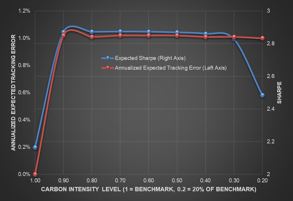
By running the optimizer and varying the carbon reduction multiplier m until the point of failure, we were able to plot the Carbon Optimized Frontier depicted in Figure 1.

From a tracking error (TE) perspective, we see that the carbon intensity can be reduced to 20% of original level (80% reduction) whilst maintaining TE around 1%. This indicates that the portfolio performance should closely track the S&P 500 benchmark index.

Figure 1. Carbon Optimized – Sharpe Ratio Frontier

^{Source: S&P Global Market Intelligence. Back tested performance has inherent limitations. The returns shown are hypothetical, do not represent the results of actual trading of investor assets, and are constructed with the benefit of hindsight. Thus, the performance shown does not reflect the impact that material economic and market factors had or might have had on decision making if actual investor money had been managed. Returns do not include payments of any sales charges or fees. Such costs would lower performance. Past performance is not a guarantee of future results. Data as of 5/12/2021.}

However, expected Sharpe Ratio slopes down gradually as we reduce the carbon intensity level with the sharpest drop happening beyond m = 0.3. This means that we can expect only a slight performance trade-off even if we reduce the carbon intensity down to 30% of original level (70% reduction).

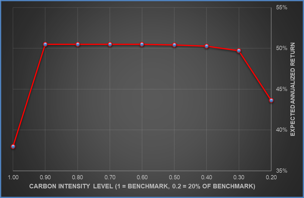
Looking at Figure 2, the performance impact of carbon reduction can be further confirmed by looking at the annualized expected return. Going from 70% to 80% of carbon reduction, we observed a -6% to negative impact on the portfolio annualized return. This is expected as the optimizer may have to shift the stock weights around significantly compared to the original, moving away from the top performers.

The tracking error, expected Sharpe, and expected annualized return will vary depending on the date of the optimization, alpha model and risk model utilized in the optimization process, as such we ask the readers not to be too concerned on the magnitude of those metrics in this article.

Figure 2. Expected Annualized Return

^{Source: S&P Global Market Intelligence. Back tested performance has inherent limitations. The returns shown are hypothetical, do not represent the results of actual trading of investor assets, and are constructed with the benefit of hindsight. Thus, the performance shown does not reflect the impact that material economic and market factors had or might have had on decision making if actual investor money had been managed. Returns do not include payments of any sales charges or fees. Such costs would lower performance. Past performance is not a guarantee of future results. Data as of 5/12/2021.}

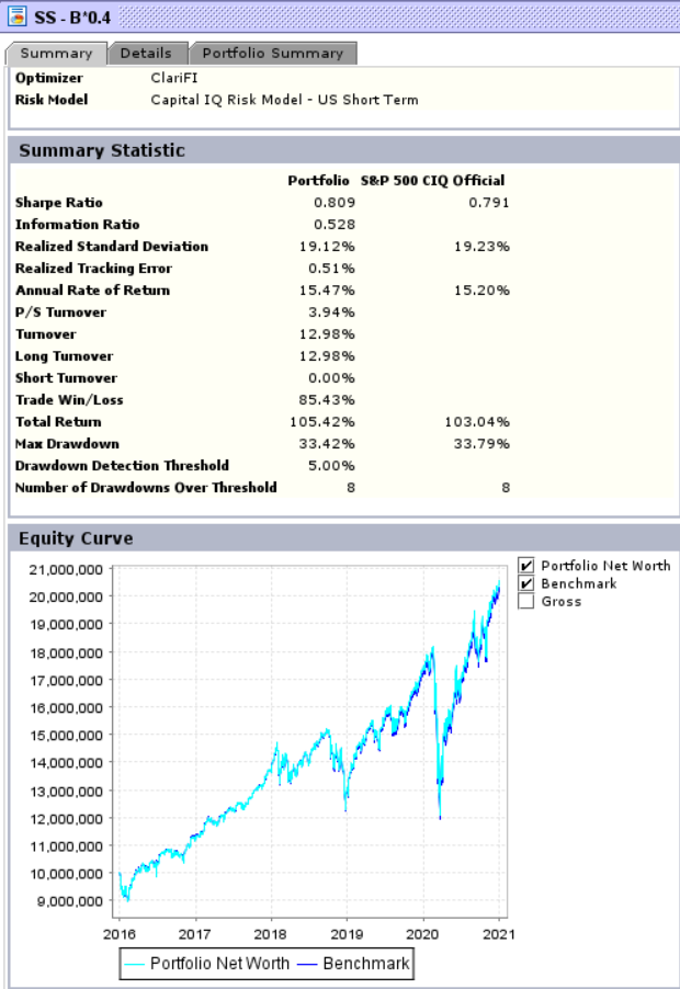
To test our hypothesis further, we extended the analysis to a 5-year historical simulation ending on December 31^st, 2020. The portfolio is rebalanced at the end of every quarter (March 31^st, June 30^th, September 30^th, and December 31^st), and the long position transaction cost is assumed to be 3bps.

Figure 3 shows a promising historical simulation result with Sharpe Ratio, volatility, drawdown, and total return tracking the benchmark S&P 500 closely with only 0.51 tracking error despite the 60% reduction in carbon intensity. Annualized turnover also stays very reasonable at 12.98%.

We are very encouraged by the back-test as we were able to maintain the performance level of the original index while reducing the carbon intensity by a significant 60% amount.

Figure 3. 5-year Historical Optimization Simulation, 60% Reduction of Carbon Intensity Scope I and II

^{Source: S&P Global Market Intelligence. Back tested performance has inherent limitations. The returns shown are hypothetical, do not represent the results of actual trading of investor assets, and are constructed with the benefit of hindsight. Thus, the performance shown does not reflect the impact that material economic and market factors had or might have had on decision making if actual investor money had been managed. Returns do not include payments of any sales charges or fees. Such costs would lower performance. Indices are unmanaged, statistical composites and their returns do not include the payment of any sales charges or fees an investor would pay to purchase the securities they represent. It is not possible to invest directly in an index. Past performance is not a guarantee of future results. Data as of 5/12/2021.}

Sector Analysis

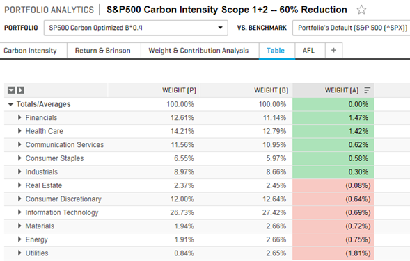
Figure 4 below depicts the 60% carbon-reduced portfolio (P) vs. benchmark (B) GICS sector weight composition. Despite having no sector weight constraints during the optimization, the optimized portfolio did not deviate from the benchmark on a sector basis as depicted by WEIGHT (A) active weight numbers.

We can see that the optimized portfolio rotates its holdings by underweighting the carbon heavy-hitter sectors (Utilities, Energy, Materials) and overweighting the lower carbon-intensive sectors (Financials, Health Care).

Figure 4. Carbon Optimized Portfolio vs. Benchmark Sector Analysis

^{Source: S&P Global Market Intelligence. Back tested performance has inherent limitations. The returns shown are hypothetical, do not represent the results of actual trading of investor assets, and are constructed with the benefit of hindsight. Thus, the performance shown does not reflect the impact that material economic and market factors had or might have had on decision making if actual investor money had been managed. Returns do not include payments of any sales charges or fees. Such costs would lower performance. Indices are unmanaged, statistical composites and their returns do not include the payment of any sales charges or fees an investor would pay to purchase the securities they represent. It is not possible to invest directly in an index. Past performance is not a guarantee of future results. Data as of 5/12/2021.}

Where do we go from here?

We have shown that it is possible to reduce a portfolio’s carbon intensity while maintaining the performance level (Sharpe, tracking error, and return) with a minimal trade-off.

The simulated Carbon Optimized Frontier demonstrates how carbon-aware investors can pick the optimal spot on the curve which maximizes the risk-reward/carbon level preferences based on investment mandates.

This article is a preliminary attempt to explore the performance impact of ESG metrics on equity portfolio investments, approaching the subject quantitatively looking at the Environmental section.

Maybe investing while saving the Earth doesn’t seem to be a mission impossible after all.